Does sustainable industrialization reduce climate vulnerability?
Setup: Install and Load Packages
required_packages <- c(
  "readxl", "dplyr", "tidyr", "ggplot2",
  "ggcorrplot", "scales", "stringr",
  "rnaturalearth", "sf"
)
new_packages <- required_packages[
  !(required_packages %in% installed.packages()[,"Package"])
]
if (length(new_packages) > 0) install.packages(new_packages)
invisible(lapply(required_packages, library, character.only = TRUE))
if (!requireNamespace("rnaturalearthdata", quietly = TRUE)) {
  install.packages("rnaturalearthdata")
}
dir.create("output_figures", showWarnings = FALSE)
Section 1: Read and Merge Data
data_path <- "Dataviz.xlsx"

panel_raw   <- read_excel(data_path, sheet = "Sheet1")
country_grp <- read_excel(data_path, sheet = "Sheet2")

panel <- panel_raw %>%
  left_join(country_grp, by = c("country" = "Country Name")) %>%
  rename(
    CVUL  = vul,  SIND = ind,  GE   = ge,
    FD    = fd,   GDPG = gdpg, TO   = to,
    POPG  = popg,
    Group = `Development Status`
  ) %>%
  select(country, year, Group, CVUL, SIND, GE, FD, GDPG, TO, POPG)

cat("Rows with missing Group:", sum(is.na(panel$Group)), "\n")
group_colors <- c("Developed" = "#2C7FB8", "Developing" = "#D95F02")
Section 2: Global Average Trend (2000–2022)
trend_global <- panel %>%
  group_by(year) %>%
  summarise(
    CVUL = mean(CVUL, na.rm = TRUE),
    SIND = mean(SIND, na.rm = TRUE)
  ) %>%
  pivot_longer(cols = c(CVUL, SIND),
               names_to = "Variable", values_to = "Value")

p_trend_global <- ggplot(
    trend_global, aes(x = year, y = Value, color = Variable)) +
  geom_line(linewidth = 1.1) +
  geom_point(size = 1.5) +
  scale_x_continuous(breaks = seq(2000, 2022, 2)) +
  scale_color_manual(
    values = c("CVUL" = "#B2182B", "SIND" = "#4575B4")) +
  labs(
    title    = "Global Average Trend: Climate Vulnerability vs. Sustainable Industrialization",
    subtitle = "Pooled average across 103 countries, 2000-2022",
    x = "Year", y = "Index value", color = NULL) +
  theme_minimal(base_size = 13) +
  theme(legend.position = "top",
        plot.title = element_text(face = "bold"))

ggsave("output_figures/01_trend_global.png",
       p_trend_global, width = 9, height = 5.5, dpi = 300)
Output ***
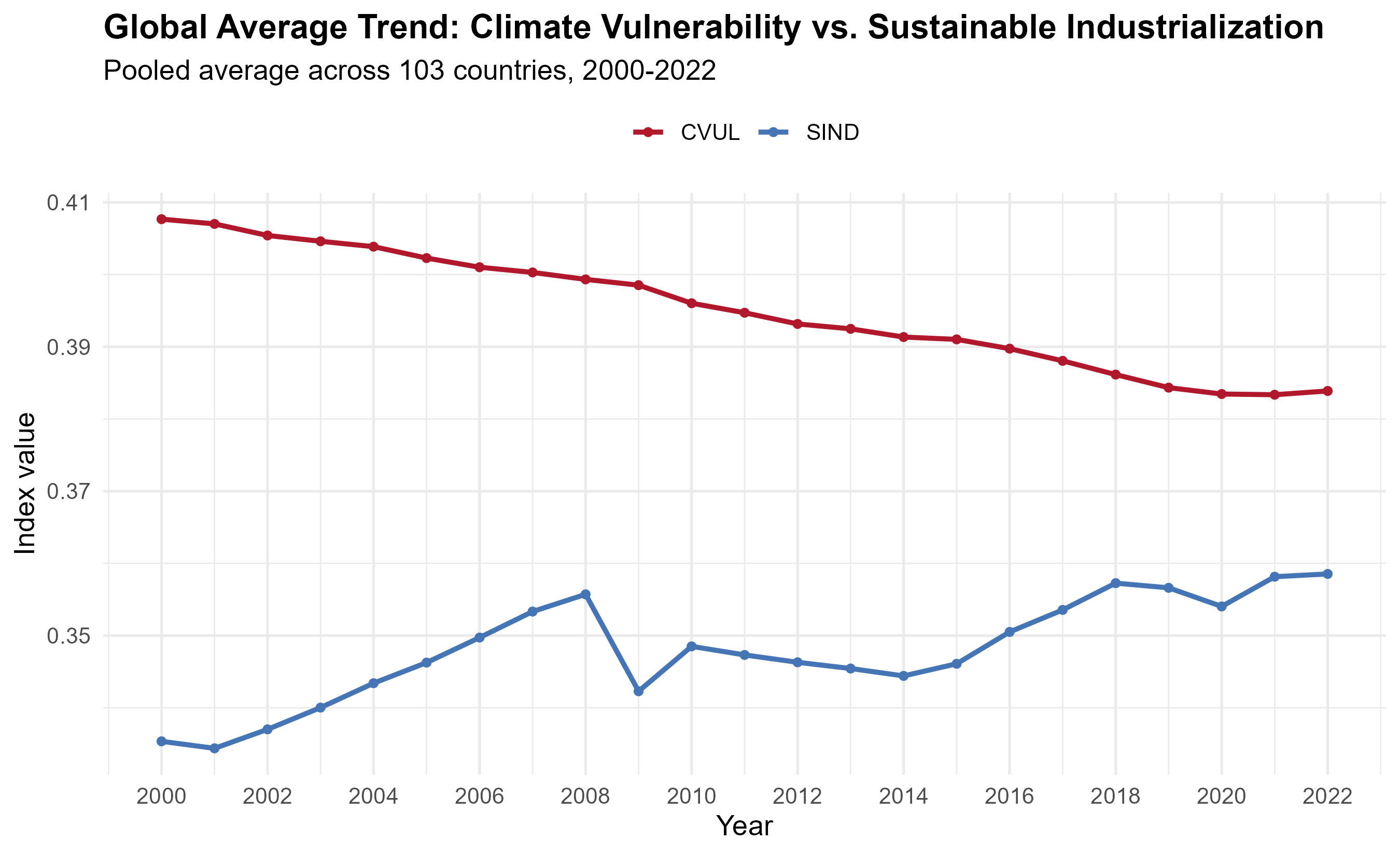 Figure 1: Global average trend of Climate Vulnerability (CVUL) and Sustainable Industrialization (SIND), 2000–2022.
Section 2b: Trend by Development Status
trend_group <- panel %>%
  group_by(year, Group) %>%
  summarise(
    CVUL = mean(CVUL, na.rm = TRUE),
    SIND = mean(SIND, na.rm = TRUE), .groups = "drop") %>%
  pivot_longer(cols = c(CVUL, SIND),
               names_to = "Variable", values_to = "Value")

p_trend_group <- ggplot(
    trend_group,
    aes(x = year, y = Value, color = Group, linetype = Variable)) +
  geom_line(linewidth = 1.1) +
  scale_x_continuous(breaks = seq(2000, 2022, 2)) +
  scale_color_manual(values = group_colors) +
  facet_wrap(~ Variable, scales = "free_y", ncol = 1,
    labeller = as_labeller(c(
      CVUL = "Climate Vulnerability (CVUL)",
      SIND = "Sustainable Industrial Index (SIND)"))) +
  labs(title = "Trends by Development Status, 2000-2022",
       x = "Year", y = "Index value",
       color = "Country group", linetype = NULL) +
  theme_minimal(base_size = 13) +
  theme(legend.position = "top",
        plot.title = element_text(face = "bold"),
        strip.text = element_text(face = "bold"))

ggsave("output_figures/02_trend_by_group.png",
       p_trend_group, width = 9, height = 7, dpi = 300)
Output ***
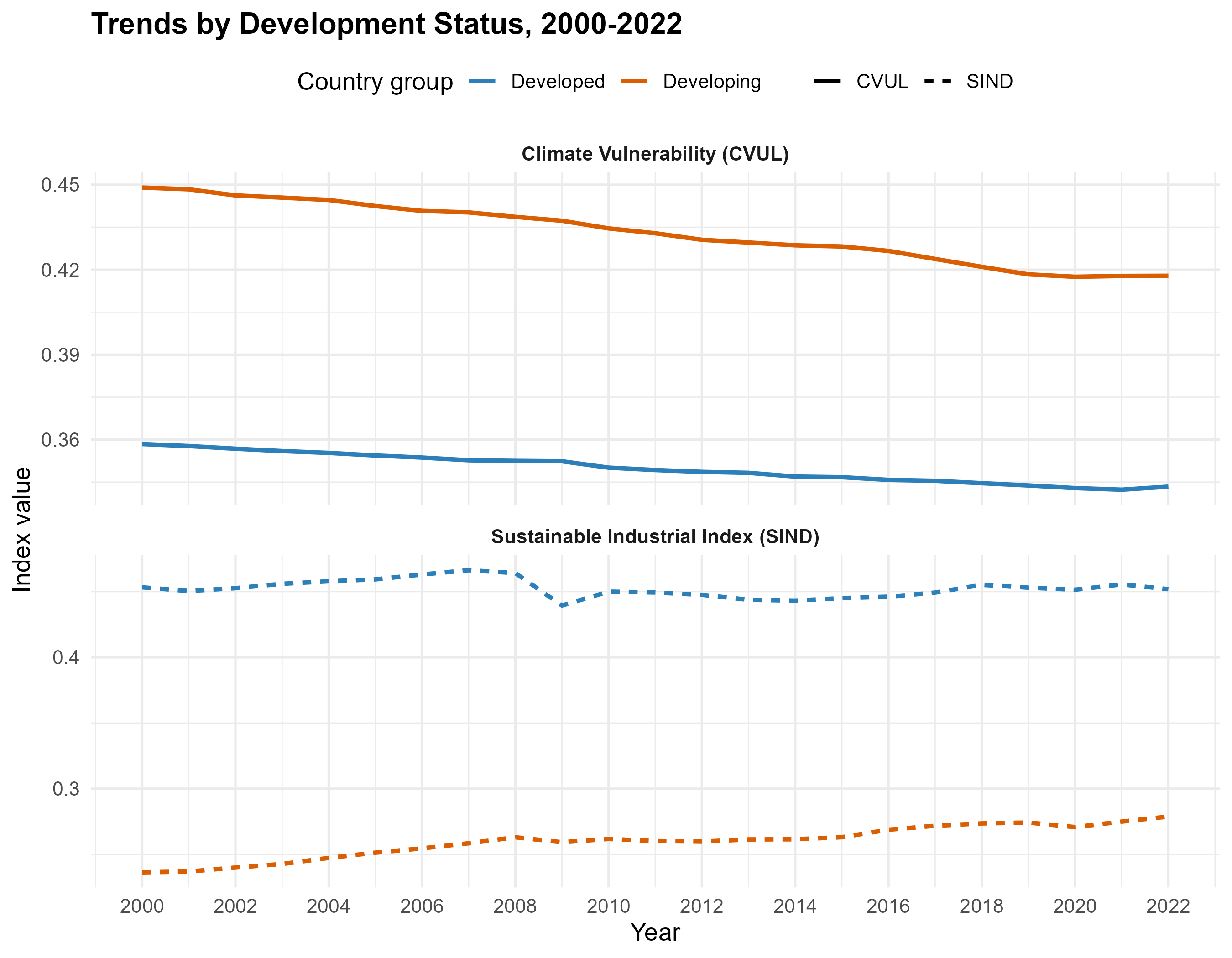 Figure 2: CVUL and SIND trends split by Developed vs. Developing countries.
Section 3: Group Comparisons (Box Plots)
vars_to_compare <- c("CVUL","SIND","GE","FD","GDPG","TO","POPG")

panel_long <- panel %>%
  select(Group, all_of(vars_to_compare)) %>%
  pivot_longer(cols = all_of(vars_to_compare),
               names_to = "Variable", values_to = "Value") %>%
  mutate(Variable = factor(Variable, levels = vars_to_compare))

p_boxplots <- ggplot(
    panel_long, aes(x = Group, y = Value, fill = Group)) +
  geom_boxplot(outlier.alpha = 0.4, width = 0.6) +
  facet_wrap(~ Variable, scales = "free_y", ncol = 4) +
  scale_fill_manual(values = group_colors) +
  labs(title = "Developed vs. Developing: Variable Comparison",
       x = NULL, y = NULL) +
  theme_minimal(base_size = 12) +
  theme(legend.position = "none",
        plot.title = element_text(face = "bold"),
        strip.text = element_text(face = "bold"))

ggsave("output_figures/03_group_boxplots.png",
       p_boxplots, width = 11, height = 6, dpi = 300)
Output ***
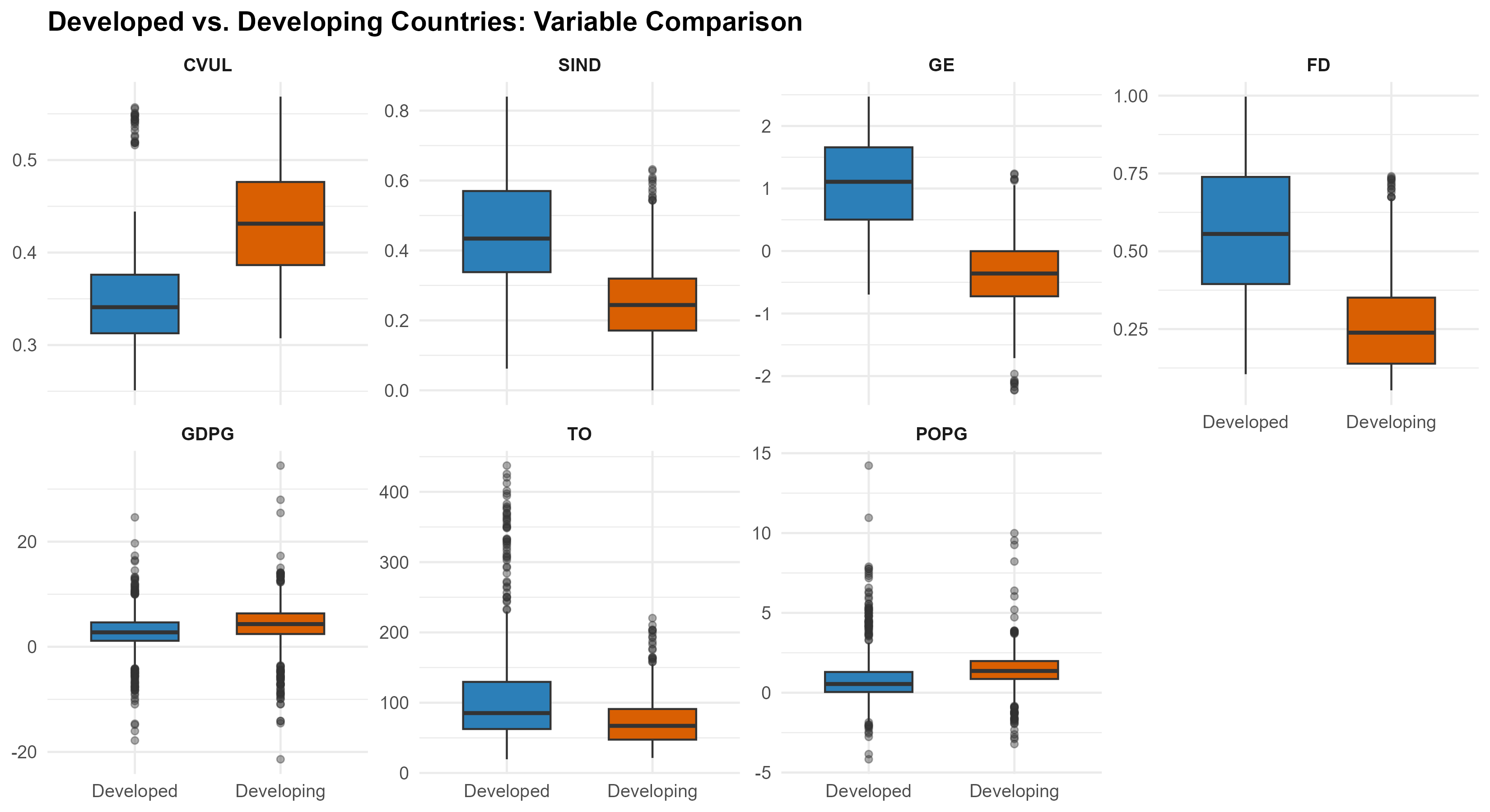 Figure 3: Distribution comparison of all study variables across country groups.
Section 4: Bivariate Relationship (CVUL vs SIND)
p_scatter <- ggplot(
    panel, aes(x = SIND, y = CVUL, color = Group)) +
  geom_point(alpha = 0.5, size = 1.8) +
  geom_smooth(method = "lm", se = TRUE,
              aes(group = Group), linewidth = 1) +
  scale_color_manual(values = group_colors) +
  labs(
    title    = "Climate Vulnerability vs. Sustainable Industrialization",
    subtitle = "Each point = one country-year (2000-2022)",
    x = "Sustainable Industrial Index (SIND)",
    y = "Climate Vulnerability Index (CVUL)",
    color = "Country group") +
  theme_minimal(base_size = 13) +
  theme(legend.position = "top",
        plot.title = element_text(face = "bold"))

ggsave("output_figures/04_scatter_cvul_sind.png",
       p_scatter, width = 8, height = 6, dpi = 300)
Output ***
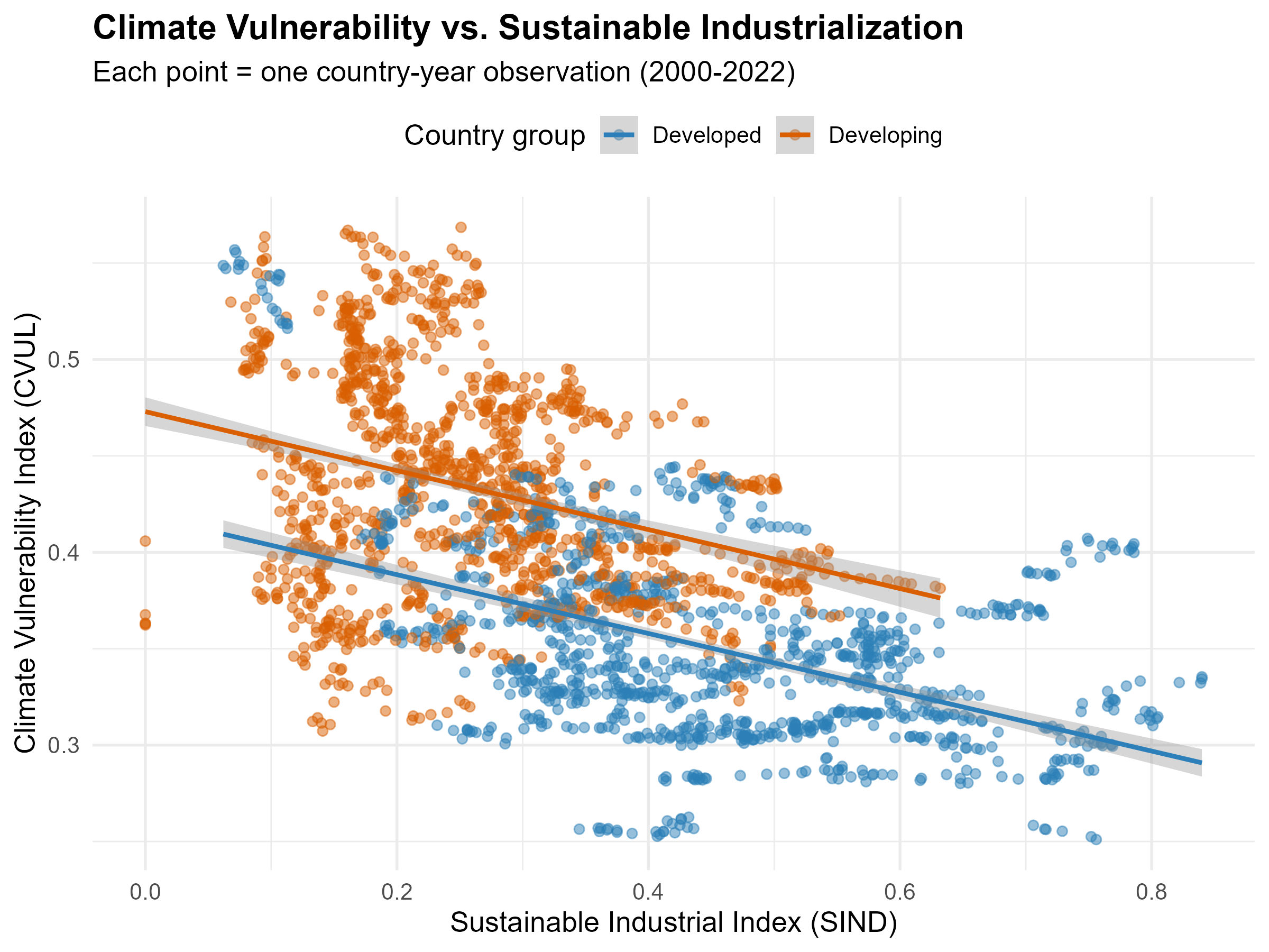 Figure 4: Scatter plot of CVUL against SIND with linear trend lines by group.
Section 5: Correlation Heatmap
corr_data   <- panel %>%
  select(all_of(vars_to_compare)) %>% na.omit()
corr_matrix <- cor(corr_data, use = "complete.obs")

p_corr <- ggcorrplot(corr_matrix,
  type    = "lower", lab = TRUE, lab_size = 3.5,
  colors  = c("#B2182B", "white", "#2166AC"),
  title   = "Correlation Matrix: Key Study Variables",
  ggtheme = theme_minimal(base_size = 13)) +
  theme(plot.title = element_text(face = "bold"))

ggsave("output_figures/05_correlation_heatmap.png",
       p_corr, width = 7, height = 6, dpi = 300)
Output ***
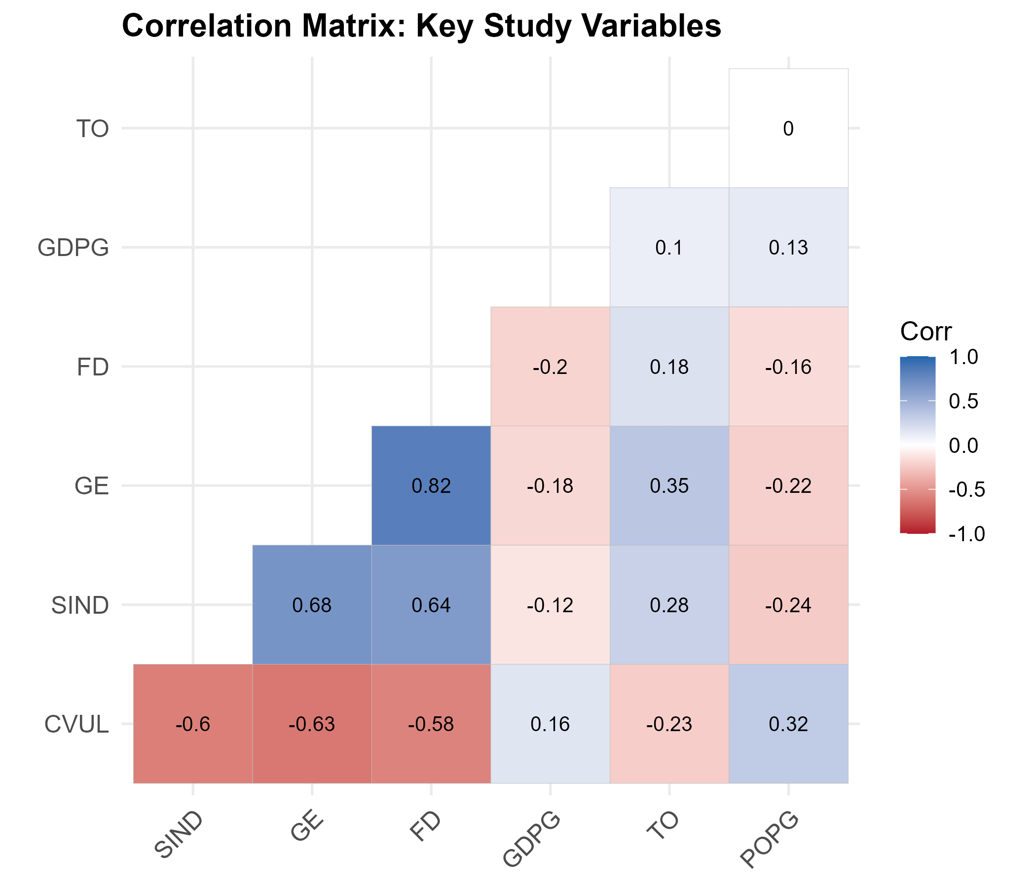 Figure 5: Correlation matrix showing pairwise relationships among study variables.
Section 6: Geographic Maps
country_avg <- panel %>%
  group_by(country) %>%
  summarise(CVUL = mean(CVUL, na.rm = TRUE),
            SIND = mean(SIND, na.rm = TRUE))

name_fix <- c(
  "Cote d'Ivoire"      = "Ivory Coast",
  "Egypt, Arab Rep."   = "Egypt",
  "Iran, Islamic Rep." = "Iran",
  "Kyrgyz Republic"    = "Kyrgyzstan",
  "Russian Federation" = "Russia",
  "Slovak Republic"    = "Slovakia",
  "Turkiye"            = "Turkey",
  "United States"      = "United States of America",
  "Viet Nam"           = "Vietnam",
  "Brunei Darussalam"  = "Brunei"
)

country_avg <- country_avg %>%
  mutate(country_map = recode(country, !!!name_fix))

world      <- ne_countries(scale = "medium", returnclass = "sf")
world_data <- world %>%
  left_join(country_avg, by = c("name" = "country_map"))

p_map_cvul <- ggplot(world_data) +
  geom_sf(aes(fill = CVUL), color = "grey40", linewidth = 0.1) +
  scale_fill_viridis_c(option = "magma", direction = -1,
                       na.value = "grey90", name = "CVUL") +
  labs(title    = "Climate Change Vulnerability Index",
       subtitle = "Country average, 2000-2022") +
  theme_minimal(base_size = 13) +
  theme(axis.text = element_blank(), axis.ticks = element_blank(),
        panel.grid = element_blank(),
        plot.title = element_text(face = "bold"))

p_map_sind <- ggplot(world_data) +
  geom_sf(aes(fill = SIND), color = "grey40", linewidth = 0.1) +
  scale_fill_viridis_c(option = "viridis",
                       na.value = "grey90", name = "SIND") +
  labs(title    = "Sustainable Industrial Index (SDG 9)",
       subtitle = "Country average, 2000-2022") +
  theme_minimal(base_size = 13) +
  theme(axis.text = element_blank(), axis.ticks = element_blank(),
        panel.grid = element_blank(),
        plot.title = element_text(face = "bold"))

ggsave("output_figures/06_map_cvul.png",
       p_map_cvul, width = 10, height = 6, dpi = 300)
ggsave("output_figures/06b_map_sind.png",
       p_map_sind, width = 10, height = 6, dpi = 300)
Output ***
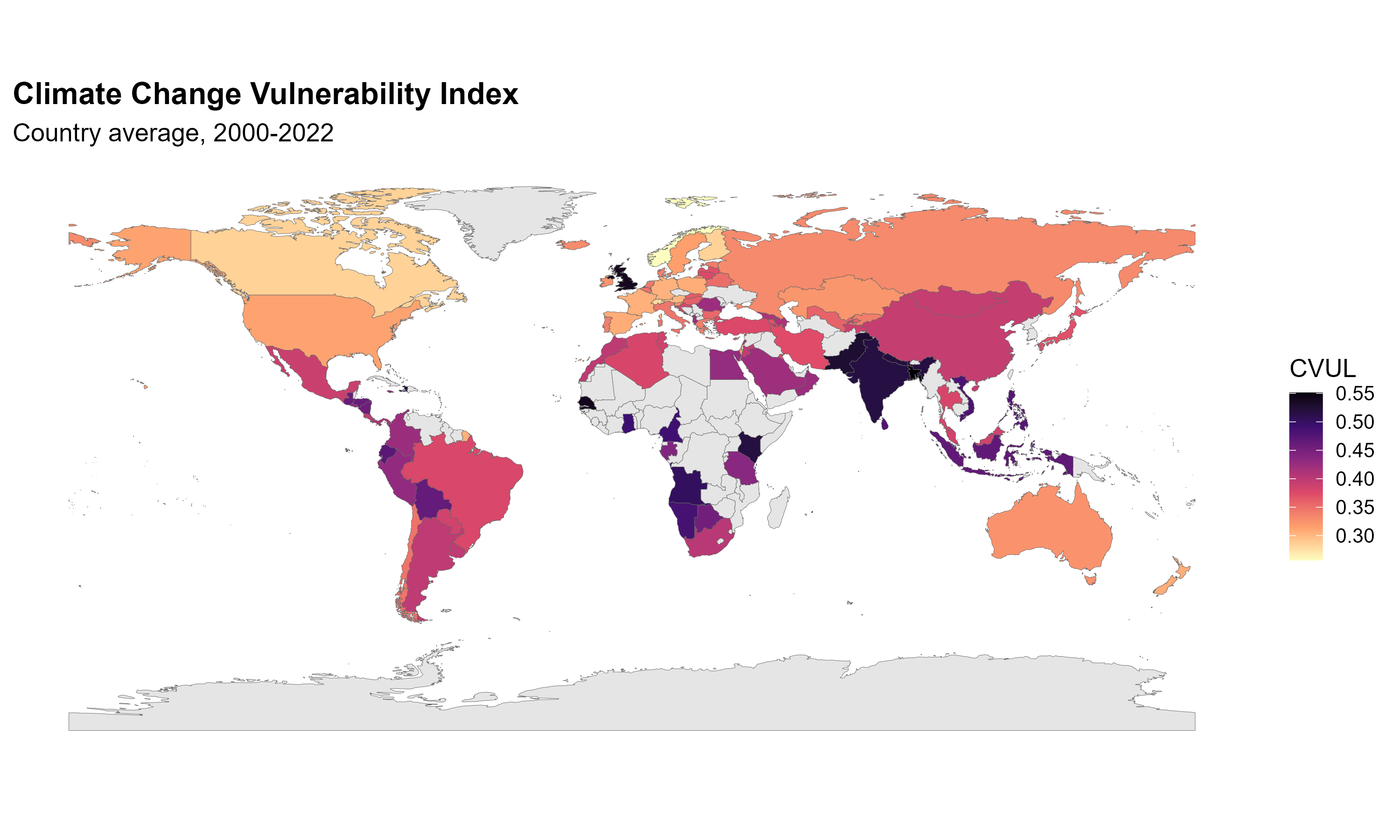 Figure 6: Global map of average Climate Vulnerability Index (CVUL), 2000–2022.
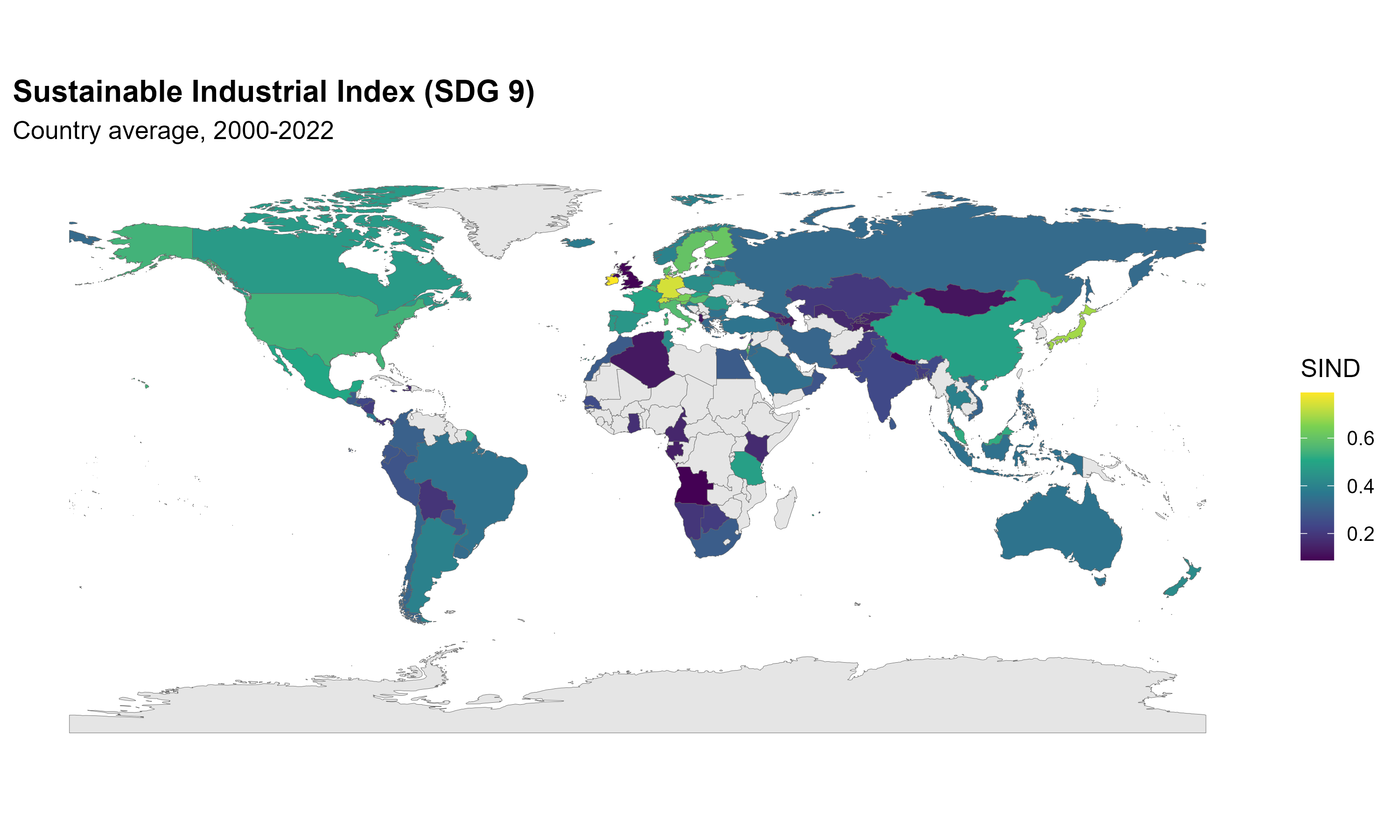 Figure 6b: Global map of average Sustainable Industrial Index (SIND), 2000–2022.
Enjoy Reading This Article?
Here are some more articles you might like to read next: